Acoustic metrology is a field for which I have no practical use. Here is an article on a homemade loudness meter.
Sound waves are longitudinal waves that propagate through the compression and rarefaction of some medium (air for the rest of this discussion). These vibrations modulate air pressure, which is what our ears and acoustic instruments detect. To put a number on these variations, we use the root mean square (RMS) value of the pressure and compare it to a reference of 20 microPascals, roughly the threshold of human hearing. Static atmospheric pressure is excluded from the calculation. This measure is known as sound pressure level (SPL) and is often expressed in decibels. For some context, 0 dB SPL is the threshold of hearing, 60 dB about a standard conversation, and sounds above 130 dB are painful and can cause immediate hearing loss.
So measuring SPL is easy and unambigous. Unfortunately, measuring loudness is not that straightforward, as it has no SI base unit nor can it be derived from base units. The culprit for this metrological transgression is psychoacoustics; to measure loudness, one must replicate the human perception of sound. Research has shown that this perception is complex and nebulous, making it challenging to pin down a unit for loudness. Strangely, the candela exists as an SI base unit for light intensity, despite its reliance on a similarly approximated response of the human eye.
Despite these challenges, several competing standards implement methods for measuring perceived loudness. One critical specification in each standard is the frequency weighting. The graph below shows the frequency response for several common standards. In the United States, the A-weighting filter is most common, while the IRU-R 468 filter is prevalent in Europe and the Commonwealth. In all filters it may be seen that our hearing sensitivity peaks between 3-6 kHz and is heavily attenuated at lower or higher frequencies.

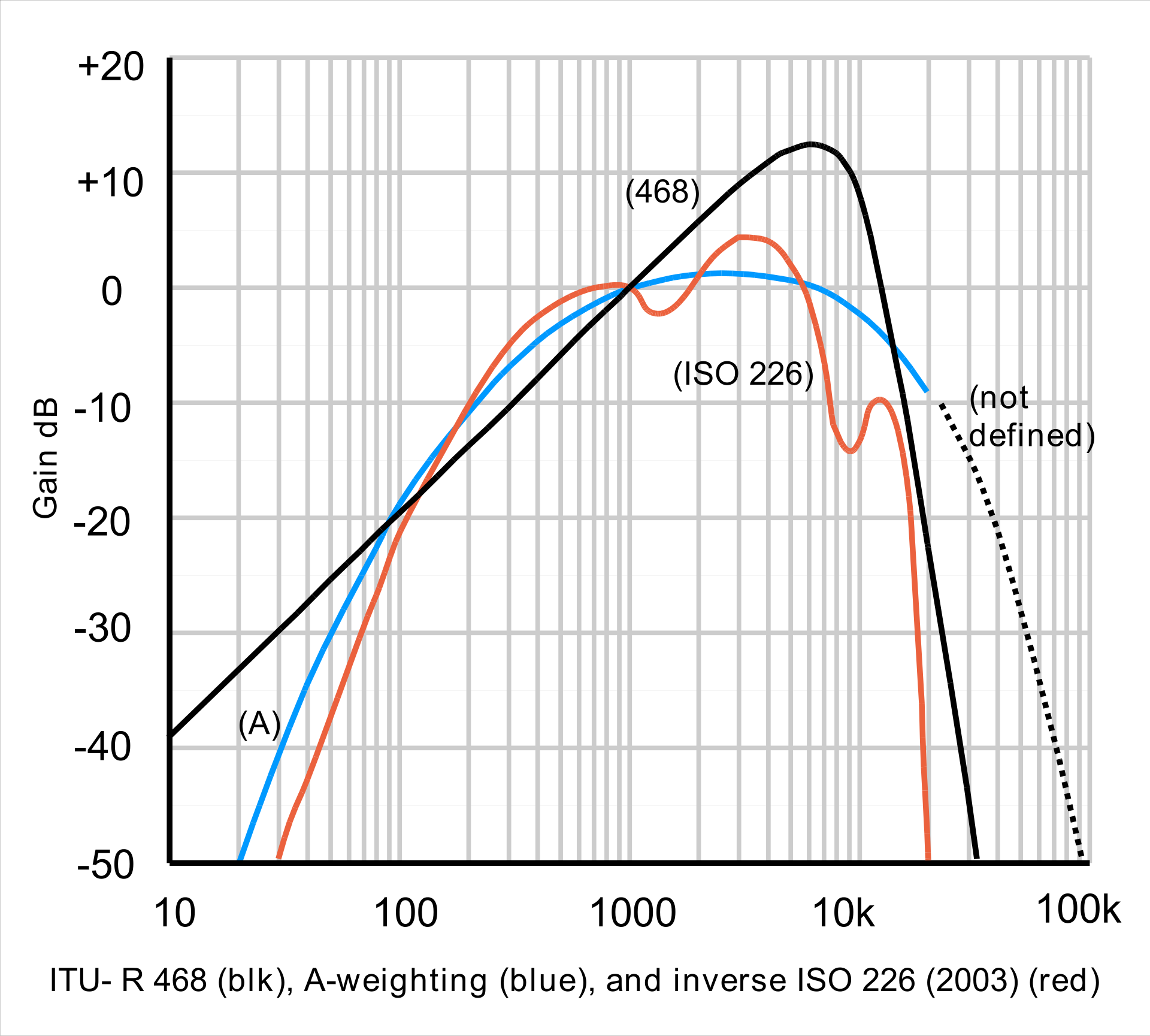
Figure 1. Lindosland. (2009). ITU-R 468 graph, A weighting, ISO 226 inverse, showing that A-weighting is similar to the equal loudness curves of human hearing for sine tones. Public Domain. Retrieved from https://commons.wikimedia.org/wiki/File:Lindos3.svg

Detection method is the other important consideration. This is the method by which the oscillating sound pressure waveform is converted to a loudness value. While SPL as a purely physical measurement uses RMS detection - as does the A-weighting specification - it has been found that human perception does not directly align with this metric (RMS measures the physical power exerted by the sound wave). The ITU-R 468 standard includes a quasi-peak detection method that approximates our increased sensitivity to short bursts of sound, but it also falls short of thoroughly replicating human hearing.
The result of this complexity is that, although we cannot implement a universally accepted loudness meter, it is still possible to take measurements of sound that reasonably reflect human-perceived loudness. The rest of this article describes an implementation of a loudness meter, its block diagram shown in Figure 2.

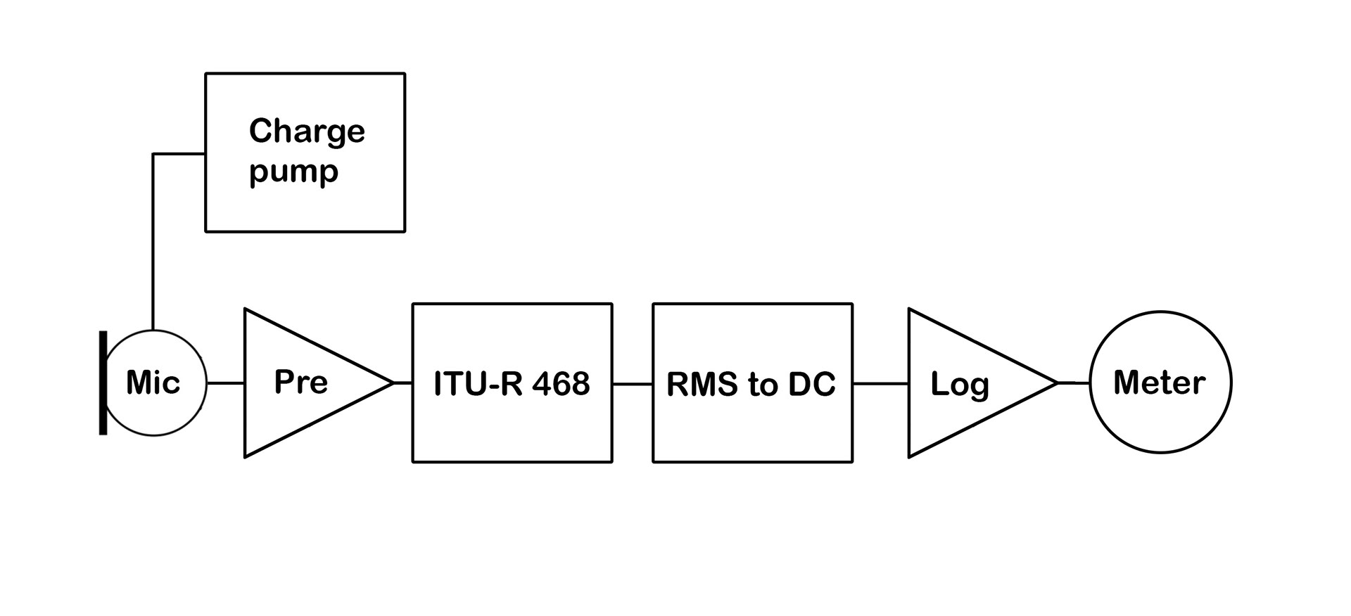
Figure 2: Block diagram of the sound level meter

The sound pressure level is sampled by a condenser microphone, its polarization voltage supplied by a charge pump. A low-noise preamplifier amplifies the microphone signal, which then passes through a filter which implements ITU-R 468 weighting. An RMS converter then produces a DC output, which is converted to decibels by a logarthmic amplifier and displayed on an analog panel meter. Figure 3 shows the hardware implementation.

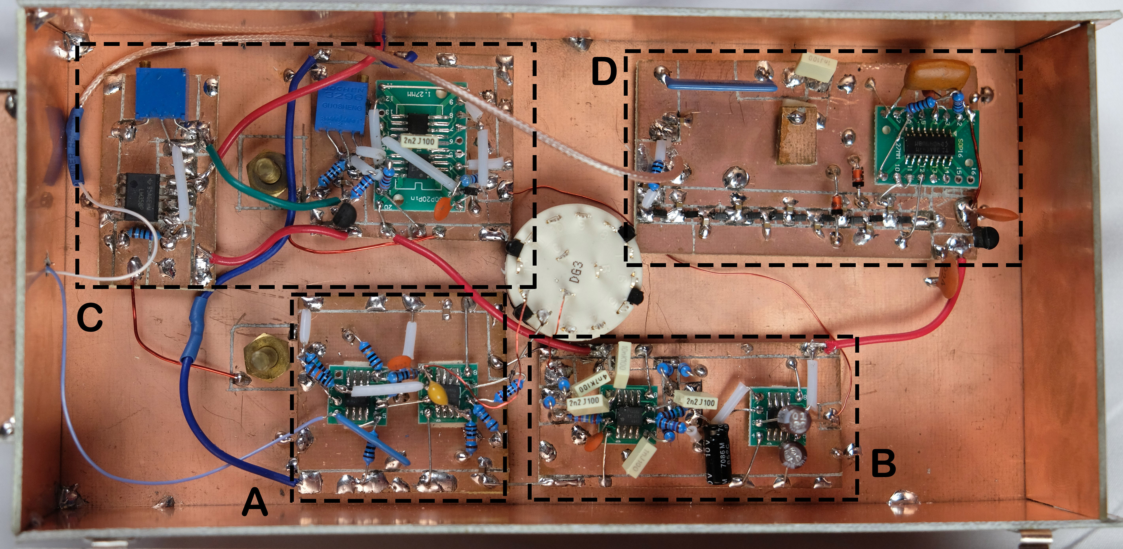
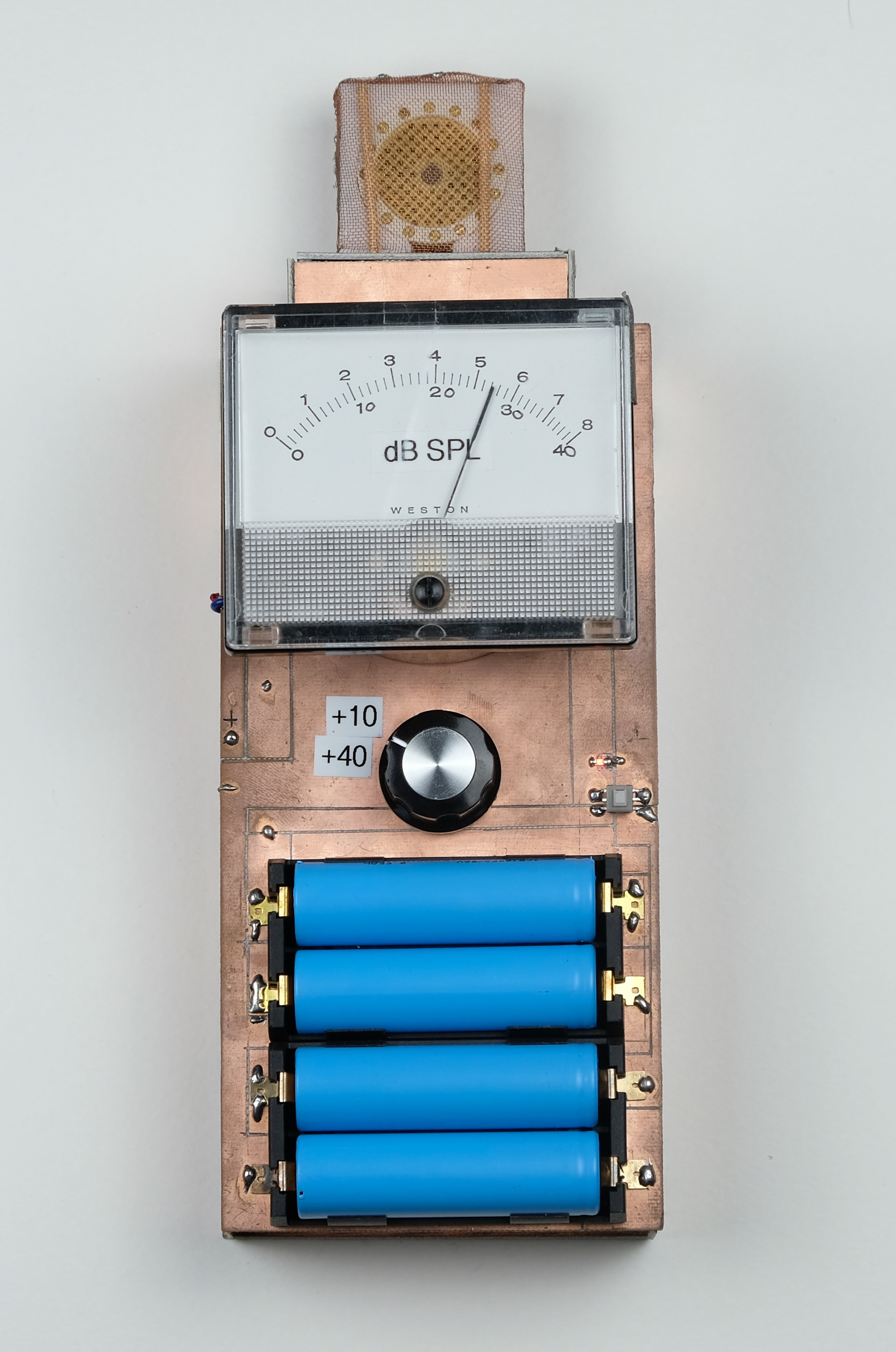
Figure 3: Sound level meter hardware implementation showing A) preamplifier; B) weighting filter and RMS-DC; C) log amplifier and meter circuitry; D) charge pump

The preamplifier (A in Fig. 3) is the most critical part of the instrument. The microphone is a condenser type, in which the vibrating diaphragm constitutes a conductive film opposing a fixed plate. Its vibrations modulate the distance between the conductors; the resulting change in capacitance produces a change in voltage provided that the stored charge on the capacitor is relatively constant (Q = CV). This implies the input impedance of the preamplifier must be large, as it forms a low-pass filter with the microphone capacitance. The TSC-1 condenser has a nominal capacitance of 56 picofarads, setting the -3dB point at 28 Hz for a 100 megaohm input impedance.
 Furthermore, the microphone has a nominal sensitivity of -35 dBV. In other words, a sound pressure level of 1 Pa (94 dB SPL) will produce -35 dBV, so at 0 dB SPL (the threshold of audition) the microphone signal will be -35 - 94 = -129 dBV, or about 350 nanovolts RMS. To keep a 350 nV signal above the noise floor over the 20-20k Hz bandwidth of the weighting filter the amplifier must have an extremely low input noise density. Just 2.5 nv/Hz^0.5, equivalent to the thermal noise on a 370 ohm resistor, would produce the same 350 nV over that bandwidth. This pair of requirements, high input impedance and low noise, informs the preamplifier design shown in Figure 4. 

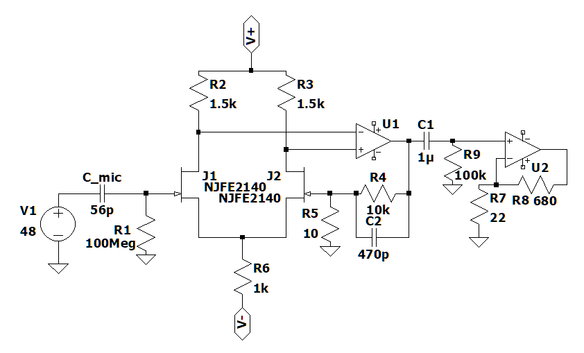
Figure 4: Preamplifier schematic

J1 and J2 form a differential input stage with R2 and R3 drain resistors and R6 setting the tail current. The transistors are Texas Instruments JFE2140 dual N-ch JFETs. These devices are extremely low noise; 1.0 nV/Hz^0.5 and 1.6 fA/Hz^0.5 input noise density. U1 (OPA2991) forms a composite amplifier with the differential pair. It provides the high open-loop gain necessary to drive the negative feedback network of R4 and R5, which linearizes the amplifier. This configuration has a simulated voltage noise density less than 2 nv/Hz^0.5. It may seem counterintuitive that, at 100 megaohms, R1's thermal noise does not dominate here. Actually, C_mic forms a low pass filter on R1's thermal noise. Increasing R1 does increase its noise, but also shifts the low pass pole left. The latter effect dominates, so increasing R1 actually decreases noise in the passband. R1 could be increased to a a gigaohm or more, but such high input impedance is very sensitive to interference and requires better shielding than currently implemented. The major contributors to passband noise are the JFETS themselves and R5. A downside of the external input stage is its high offset voltage, which must be trimmed manually by a potentiometer on one of the drain resistors.  An additional 30dB of gain is provided by U2. The rotary switch on the instrument selects between the output of U1 and U2 for the input of the weighting filter. Its schematic is illustrated in Figure 5.

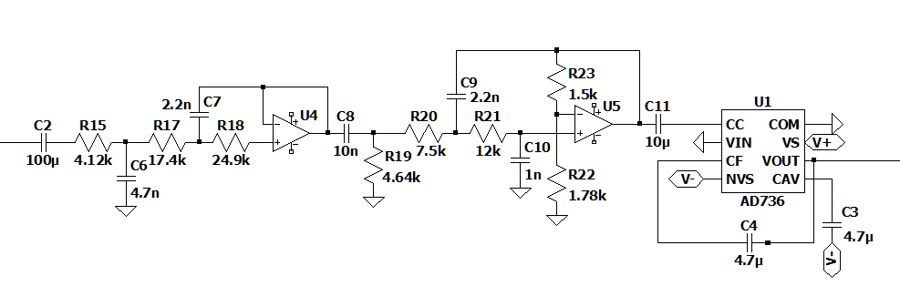
Figure 5: Weighting filter and RMS-DC converter.  Beis, Ewe. "Weighting Filter Set." October 2015. Web. 25 Apr. 2024. <https://www.beis.de/Elektronik/AudioMeasure/WeightingFilters.html>.

The 468 weighting filter is implemented by U4 and U5. An implementation of the weighting filter transfer function using E96 components is generously provided by Ewe Beis. The transfer function has one zero and 4 poles, with maximum gain at 2 kHz. The signal passes to an AD736 RMS to DC converter. Computing RMS mathematically requires squaring, integration, and square rooting. The nonlinear operations are hard to perform electronically and require excellent transistor matching for good accuracy, leaving this task best suited to an integrated circuit. C3 and C4 configure the RMS settling time to about 100 milliseconds.

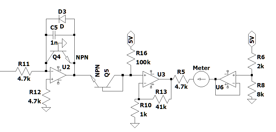
Figure 6: Log amp and meter conditioning

Figure 6 shows the logarithmic amplifier and meter circuitry. The signal current enters at R11 and passes through Q4, which provides the exponential current-voltage curve that performs the logarithmic conversion. Q5 provides an offset voltage which sets a zero voltage output when the input current equals the current through R16. These transistors are in a dual package, lending them good inherent and thermal matching. The gain of U3 and the output voltage at U6 condition the signal to match the span and the full-scale current of the meter respectively. Here the meter requires 1 mA for full deflection. The log amplifier is inverting, so at maximum input (when the input current equals R16's current) U3 outputs 0 volts. With no or minimal input current U3 saturates at the positive rail. Potentiometers (not drawn) facilitate adjustment such that a 2 decade input current range matches the 0 to 40 dB scale on the meter.

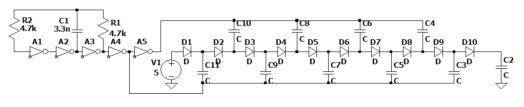
Figure 7: Dickson charge pump

The last section of circuitry in the instrument is the charge pump, responsible for the 45 volt polarizing voltage on the microphone. It is a tuned ring oscillator made from a hex inverter that oscillates at about 40 kHz. The oscillator produces complementary outputs which drive a Dickson charge pump. Each diode / capacitor pair adds one additional Vin, minus the diode forward voltage. The output voltage is then directly dependent on the input voltage V1. Because the microphone sensitivity is proportional to this voltage, the stability of the instrument depends on the stability of this polarizing voltage. The input is provided by a 5V regulator so that battery discharge does not influence the output voltage.

You may also like

Back to Top